R Code
Hello, I’m Katie! I made this website using R Markdown!
About this page:
- I made this R Markdown website to demonstrate and teach R skills
- It looks basic right now, because it is a work in progress
- My first project was a PCA one, see below
- I plan to add more advanced models as time goes by
- Check back regularly to join me on my data science journey
Disclaimer: Code and stat tips originate from my experience in academic research. Always remember to use reliable literature (language documentation, published text books, academic research papers, your own class notes) and fact check when using a website as a resource. I will try to keep everything as accurate as possible, but feel free to contact me if you have any questions on facts, figures and references. I hope you find this page useful! Enjoy!
Let’s get started!
knitr::opts_chunk$set(echo = TRUE) #Setting this equal to true allows the code to show up on the pagelibrary(tidyverse) #Includes packages such as; ggplot2, dplyr, tibble and moregetwd()## [1] "/Users/katiedunne/Documents/April2021/R_April2021/RMarkdown1"Demo of basic R skills 1
# Vector
a_vector <- c(3, 4)
a_vector
## [1] 3 4Demo of basic R skills 2
# Matrix
a_matrix <- matrix(c(1, 2, 3, 4),nrow =2, ncol=2)
a_matrix
## [,1] [,2]
## [1,] 1 3
## [2,] 2 4Demo of PCA on iris data
PCA reference: Statistics class notes combined with my own opinions and interpretation
PCA is useful for dimention reduction and identifying drivers
data(iris)
# View(iris)summary(iris)## Sepal.Length Sepal.Width Petal.Length Petal.Width
## Min. :4.300 Min. :2.000 Min. :1.000 Min. :0.100
## 1st Qu.:5.100 1st Qu.:2.800 1st Qu.:1.600 1st Qu.:0.300
## Median :5.800 Median :3.000 Median :4.350 Median :1.300
## Mean :5.843 Mean :3.057 Mean :3.758 Mean :1.199
## 3rd Qu.:6.400 3rd Qu.:3.300 3rd Qu.:5.100 3rd Qu.:1.800
## Max. :7.900 Max. :4.400 Max. :6.900 Max. :2.500
## Species
## setosa :50
## versicolor:50
## virginica :50
##
##
## fit = prcomp(iris[,1:4])
fit## Standard deviations (1, .., p=4):
## [1] 2.0562689 0.4926162 0.2796596 0.1543862
##
## Rotation (n x k) = (4 x 4):
## PC1 PC2 PC3 PC4
## Sepal.Length 0.36138659 -0.65658877 0.58202985 0.3154872
## Sepal.Width -0.08452251 -0.73016143 -0.59791083 -0.3197231
## Petal.Length 0.85667061 0.17337266 -0.07623608 -0.4798390
## Petal.Width 0.35828920 0.07548102 -0.54583143 0.7536574round(fit$rotation, 2)## PC1 PC2 PC3 PC4
## Sepal.Length 0.36 -0.66 0.58 0.32
## Sepal.Width -0.08 -0.73 -0.60 -0.32
## Petal.Length 0.86 0.17 -0.08 -0.48
## Petal.Width 0.36 0.08 -0.55 0.75The magnitude of the loadings are important, however the signs on the loadings are arbitrary. It matters if the loadings have opposite signs, but not which is positive and which is negative.
In PC1, Sepal.length, Petal.Length and Petal.Width all have large positive loadings, whereas Sepal.Width has a negative loading which is close to zero.
We could interpret the first PC as an overall measure of the ‘size’ of the flower. The sepal width variable has close to zero loading.
PC2 is contrasting flowers that have large sepals against flowers that have long petals.
summary(fit)## Importance of components:
## PC1 PC2 PC3 PC4
## Standard deviation 2.0563 0.49262 0.2797 0.15439
## Proportion of Variance 0.9246 0.05307 0.0171 0.00521
## Cumulative Proportion 0.9246 0.97769 0.9948 1.00000With regard to the code chunk above, it is important to note that the value of a particular eigenvalue divided by the sum of the eigenvalues is called the proportion of variance explained by that principal component (REF: A past statistics class)
# We can plot the proportion of variance explained by each PC using:
plot(fit, main = "Scree plot", xlab = "Comps 1:4")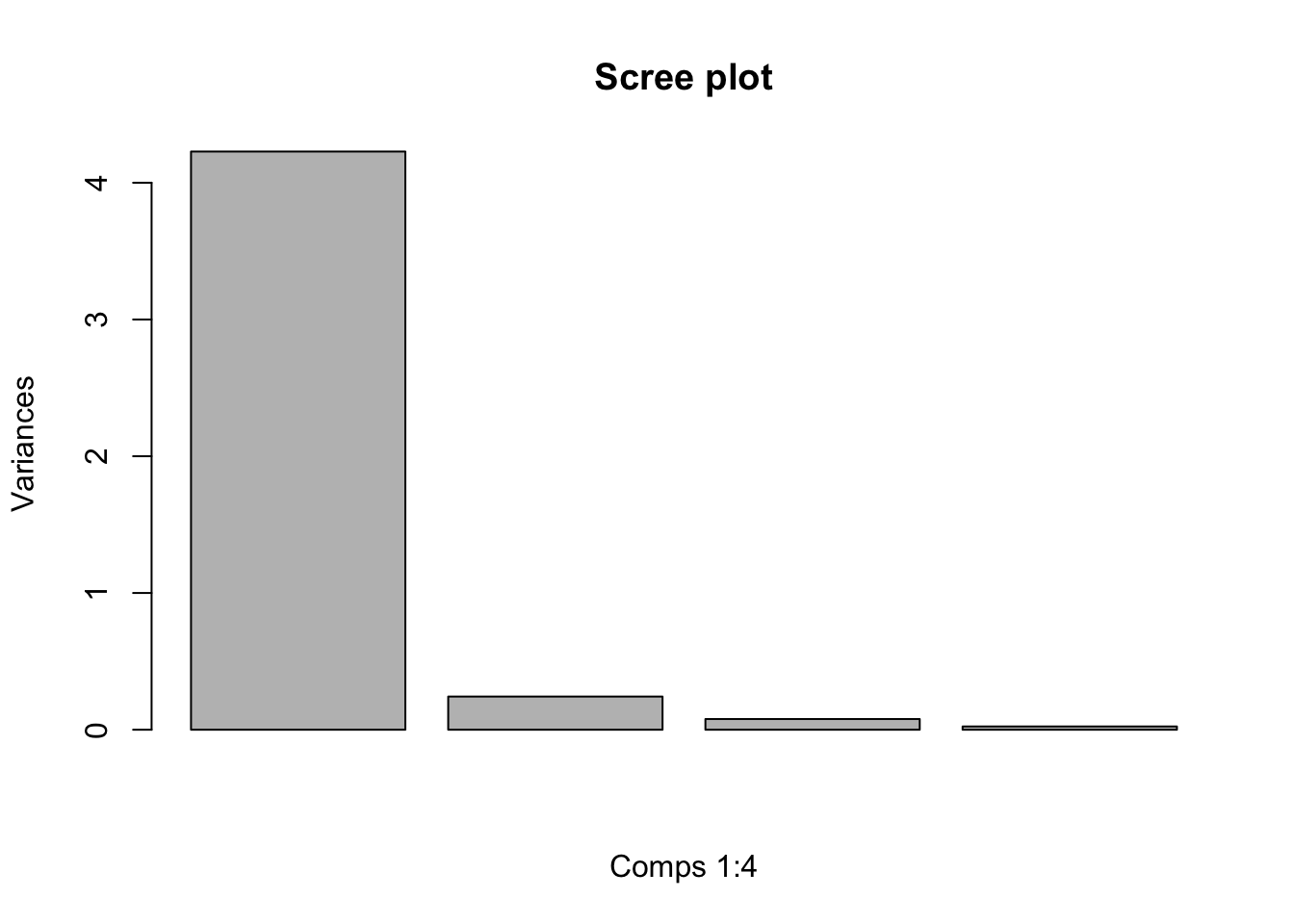
newiris = predict(fit)
newiris
To get a ‘picture’ of the reduced dimensional data we often produce a scatter plot of the scores on one PC against the scores on another PC. As we have decided that only PC1 (and maybe PC2) need to be considered we can use the plot function to plot the values of PC1 against PC2 (REF: A past statistics class)
plot(newiris[,1], newiris[,2], type="n", xlab="PC1", ylab="PC2")
text(newiris[,1], newiris[,2], labels=substr(iris[,5],1,2), col=as.integer(iris[,5]))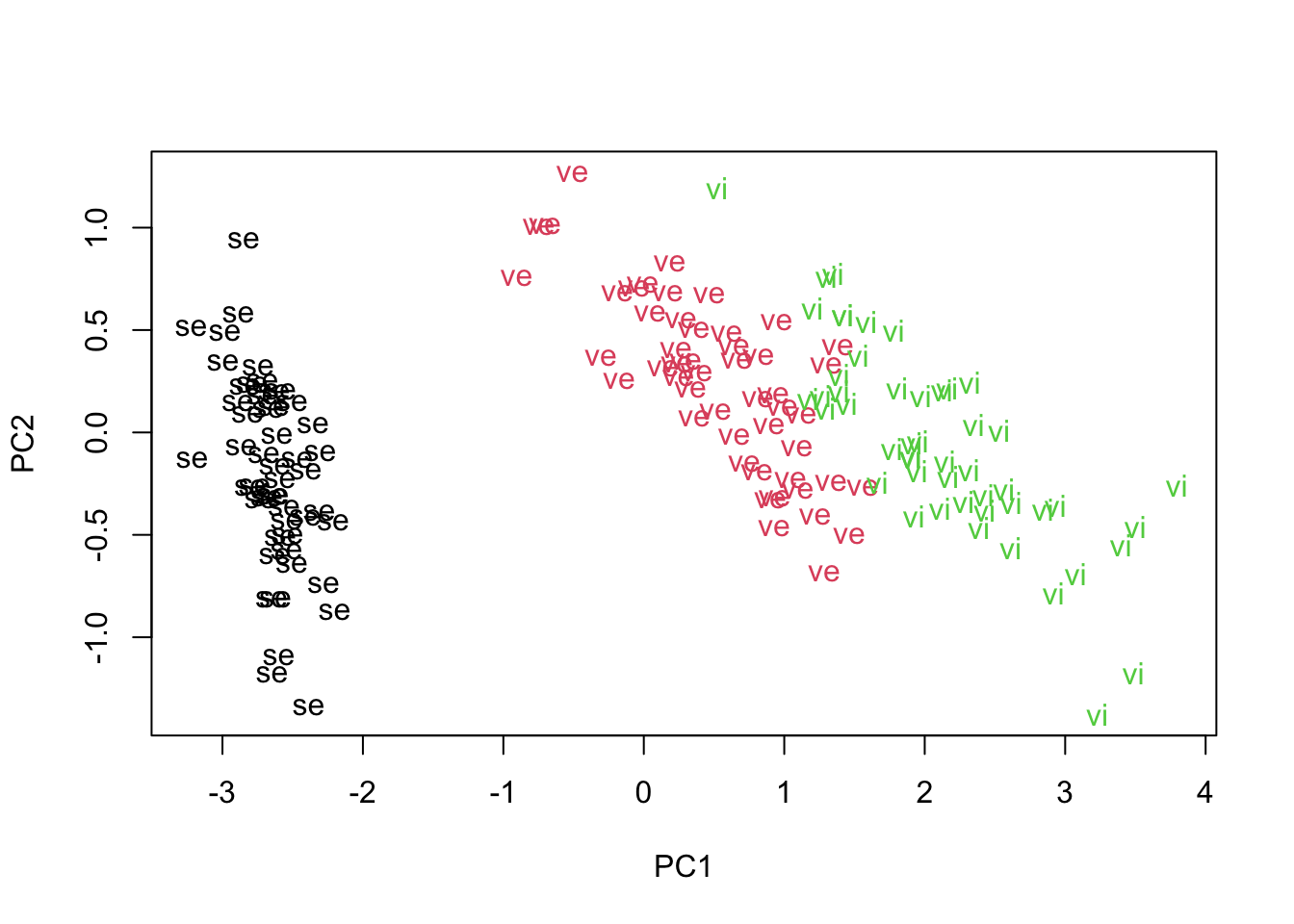
You will notice that we have performed PCA on the unstandardised data. Sometimes the data are standardised before performing PCA (REF: A past statistics class)
© 2021 Katie S. Dunne